When Your Distribution Looks All Skewed Up
Skewness is a measure of the degree of asymmetry of a distribution of numbers. Let’s take a look at an approach to quantify it.
Consider a population of size \(N\) in which the values of the random variable $Y$ are $y_1, y_2, \ldots, y_N$. The “centered population moment of order 3” is defined as:
\[\nonumber M_3 = \frac{1}{N}\sum_{i = 1}^{N}(y_i - \mu)^3\]where $\mu$ is the population mean. $M_3$ reflects the skewness of the population distribution.
The (standardized) population coefficient of skewness is denoted by $\kappa_3$ (“kappa sub 3”) and defined by:
\[\nonumber \kappa_3 = \frac{M_3}{\sigma^3}\]where $\sigma$ is the population standard deviation. By construction, this measure is not affected either by the mean of the population or by the standard deviation of the population. In symmetric distributions, $\kappa_3 = 0$. In right-skewed distributions, $\kappa_3 > 0$ and in left-skewed distributions, $\kappa_3 < 0$. As a rule of thumb, we have:
- If $\kappa_3$ is less than -1 or greater than 1, then the distribution is highly skewed;
- If $\kappa_3$ is between -1 and -0.5 or between 0.5 and 1, then the distribution is moderately skewed;
- If $\kappa_3$ is between -0.5 and 0.5, then the distribution is approximately symmetric.
$\kappa_3$ can be estimated using sample data. Simply replace the population mean $\mu$ with the sample mean $\bar{Y}$, and the population standard deviation $\sigma$ with the sample standard deviation $S$ (using the sample size $n$, not $n - 1$, in the denominator). The estimate is denoted as $\widehat{\kappa}_3$, the sample coefficient of skewness. Please note that a more formal procedure can be developed to test whether $\widehat{\kappa}_3$ is significantly different from 0.
To compute $\widehat{\kappa}_3$ is easy to do in R. One can code their own function or use a package. The skewness() function in the EnvStats package computes the sample coefficient of skewness as described above by invoking the so-called “moment” option. For example, consider the following toy data set:
> library(EnvStats)
> my_data <- c(1,1,1,1,1,2,2,2,2,3,3,3,4,4,5)
To compute $\widehat{\kappa}_3$, we do:
> skewness(my_data, method = "moment")
Following is a histogram displaying the data:
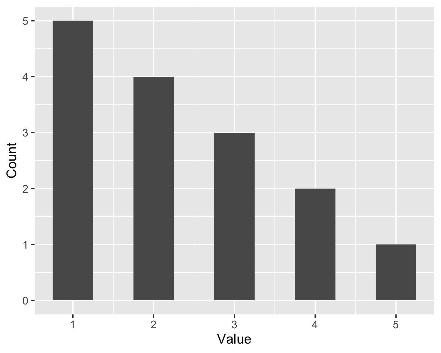
We obtain $\widehat{\kappa}_3 = 0.59$. By the rules of thumb, we have moderate right-skew.
By using the statistic $\widehat{\kappa}_3$, we can look for a departure from symmetry, how the departure manifests itself, and the strength of the departure. It provides some quantitative rigor as a companion to a histogram and therefore can be a useful tool in practice. For example, I have used this in a marketing setting where there was interest to see how sales managers differed with respect to rating assessments of their teams. Perhaps you will find an application in your future, too.